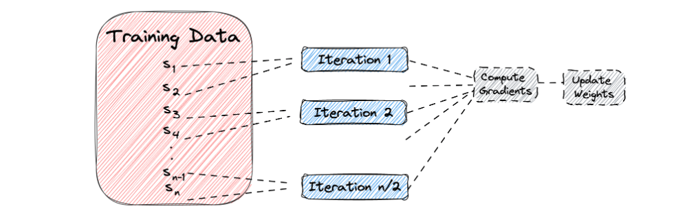
데이터 로더(Data Loader)
- 데이터의 양이 많은 때 배치 단위로 학습하는 방법을 제공한다.
손글씨 인식 모델 만들기
더보기

결과

결과
결과

결과

결과
결과

결과
결과

결과

결과

결과

결과
# 필요한 모듈 import
import torch
import torch.nn as nn
import torch.optim as optim
import matplotlib.pyplot as plt
from sklearn.datasets import load_digits
from sklearn.model_selection import train_test_split
# device 확인
device = "cuda" if torch.cuda.is_available() else "cpu"
print(device)
# 사용할 데이터를 객체에 담아준다.
digits = load_digits()

X_data = digits["data"]
y_data = digits["target"]

print(X_data.shape)
print(y_data.shape)
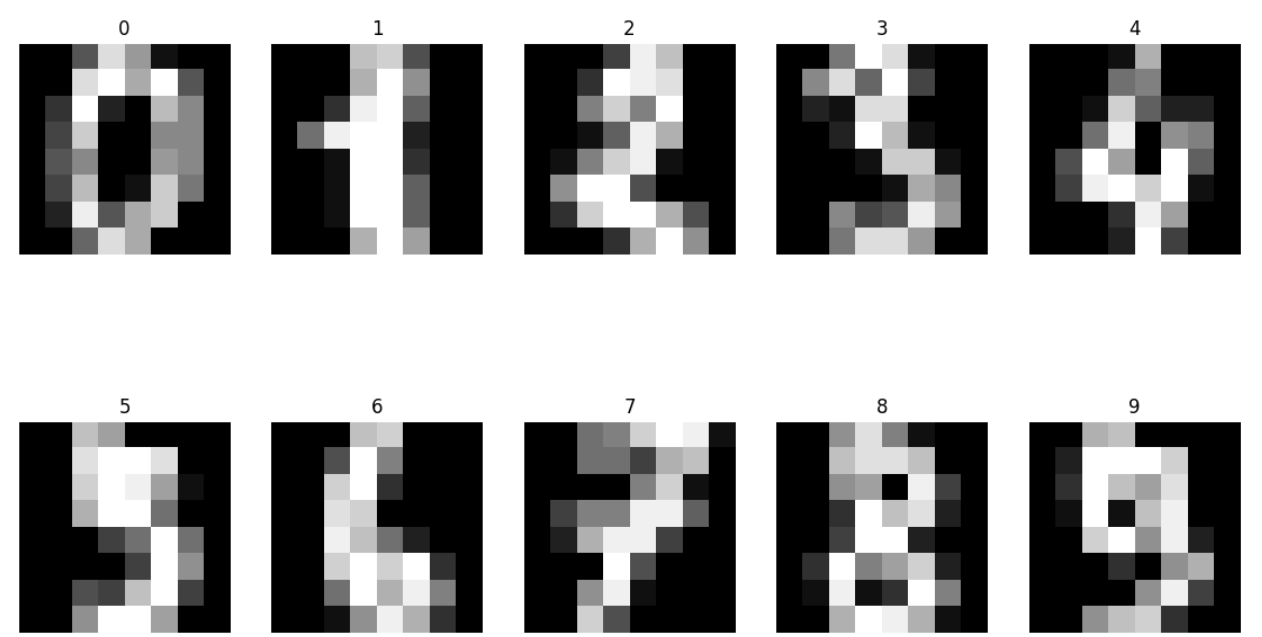
# 손글씨 데이터 뽑아보기
fig, axes = plt.subplots(nrows=2, ncols=5, figsize=(14, 8))

for i, ax in enumerate(axes.flatten()): # flatten으로 1차원으로 변경
  ax.imshow(X_data[i].reshape((8, 8)), cmap="gray") # reshape으로 8x8 2차원 배열로 변환
  ax.set_title(y_data[i]) # 현재 레이블을 제목으로 설정
  ax.axis("off") # 눈금과 라벨을 숨김
# Tensor 형태로 변환
X_data = torch.FloatTensor(X_data)
y_data = torch.LongTensor(y_data)

print(X_data.shape)
print(y_data.shape)
# 훈련/테스트 데이터로 분류
x_train, x_test, y_train, y_test = train_test_split(X_data, y_data,
                                                    test_size=0.2,
                                                    random_state=2024)
print(x_train.shape, y_train.shape)
print(x_test.shape, y_test.shape)
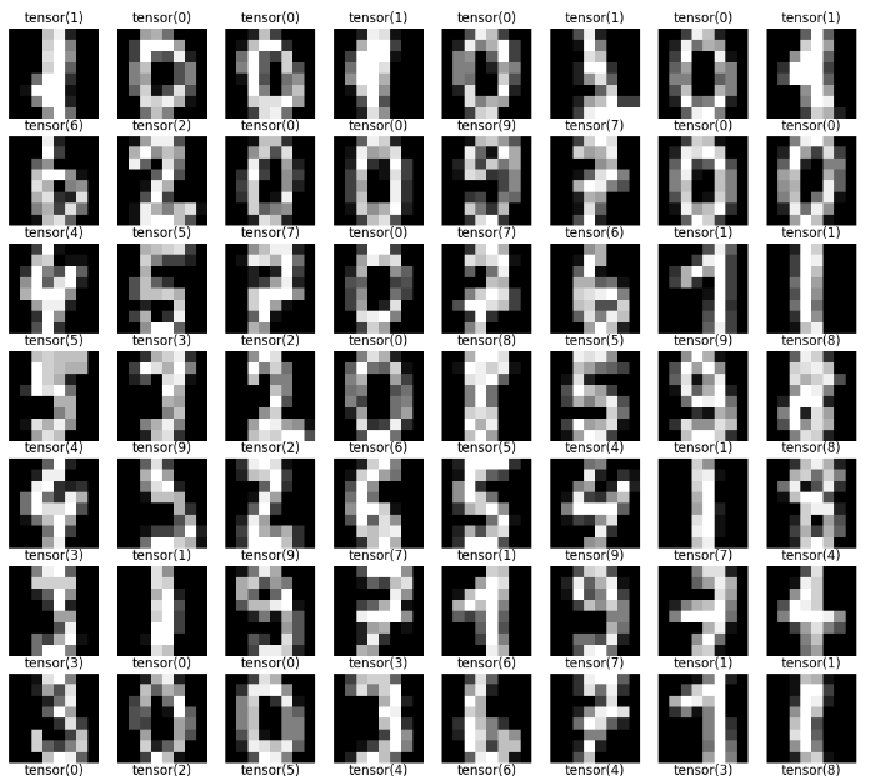
loader = torch.utils.data.DataLoader(
    dataset = list(zip(x_train, y_train)), # list로 넣어야함
    batch_size = 64, # 한 번에 로드할 데이터의 크기는 64
    shuffle = True, # 각 epoch 마다 데이터셋을 랜덤으로 섞는다.
    drop_last = False # False가 기본값, 마지막 배치를 버리지 않는다.
)

imgs, labels = next(iter(loader))
fig, axes = plt.subplots(nrows=8, ncols=8, figsize=(14, 14))

for ax, img, label in zip(axes.flatten(), imgs, labels):
  ax.imshow(img.reshape((8, 8)), cmap="gray")
  ax.set_title(str(label))
  ax.axis("off")
# 모델 생성
model = nn.Sequential(
    nn.Linear(64, 10)
)

# 최적화 계산을 위한 함수
optimizer = optim.Adam(model.parameters(), lr=0.01)

# 반복 횟수
epochs = 50

# 반복문을 사용하여 학습
for epoch in range(epochs+1):
  sum_losses = 0
  sum_accs = 0

  for x_batch, y_batch in loader:
    y_pred = model(x_batch)
    loss = nn.CrossEntropyLoss()(y_pred, y_batch)

    optimizer.zero_grad()
    loss.backward()
    optimizer.step()

    sum_losses = sum_losses + loss

    y_prob = nn.Softmax(1)(y_pred)
    y_pred_index = torch.argmax(y_prob, axis=1)
    acc = (y_batch == y_pred_index).float().sum() / len(y_batch) * 100
    sum_accs = sum_accs + acc

  avg_loss = sum_losses / len(loader)
  avg_acc = sum_accs / len(loader)
  print(f"Epoch: {epoch:4d}/{epochs} Loss: {avg_loss:.6f} Accuracy: {avg_acc:.2f}")
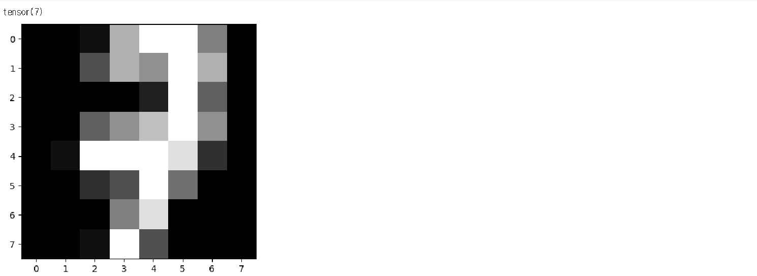
# 테스트 데이터 값 하나 확인해보기
plt.imshow(x_test[10].reshape((8, 8)), cmap="gray")
print(y_test[10])
# 예측
y_pred = model(x_test)
y_pred[10]
# 예측값과 확률
y_prob = nn.Softmax(1)(y_pred)
y_prob[10]
# 확률 확인해보기
for i in range(10):
  print(f"숫자 {i}일 확률: {y_prob[10][i]:.2f}")
y_pred_index = torch.argmax(y_prob, axis=1)
accuracy = (y_test == y_pred_index).float().sum() / len(y_test) * 100
print(f"테스트 정확도는 {accuracy: .2f}% 입니다.")
'Python > 머신러닝, 딥러닝' 카테고리의 다른 글
| Python 딥러닝 비선형 활성화 함수 (0) | 2024.06.24 |
|---|---|
| Python 딥러닝 (0) | 2024.06.24 |
| Python 머신러닝, 딥러닝 파이토치로 구현한 논리회귀 (0) | 2024.06.24 |
| Python 머신러닝, 딥러닝 파이토치로 구현한 선형 회귀 (0) | 2024.06.18 |
| Python 머신러닝, 딥러닝 파이토치 (0) | 2024.06.18 |